
Introduction
(This is for Daniel, who needs help with his Excel...)
A couple of years ago, Microsoft introduced dynamic arrays in Excel. Almost four years later, I still don't see many people using them in Office 365. (I'm working on that.)
A dynamic array can return values that populate numerous continuous cells. It is best used on a table or continuous cells (range). You can filter, sort, create a sequence, determine unique values, and do other very helpful tasks on a range of data. Once you start using dynamic arrays, you will be amazed.
Let's get some data...
I usually work with a lot of data that is in a table format. The data doesn't have to be in an Excel Table, but the data is continuous. The data doesn't have blank columns or rows. Instead of creating a bunch of data, let's pull some from a public database.
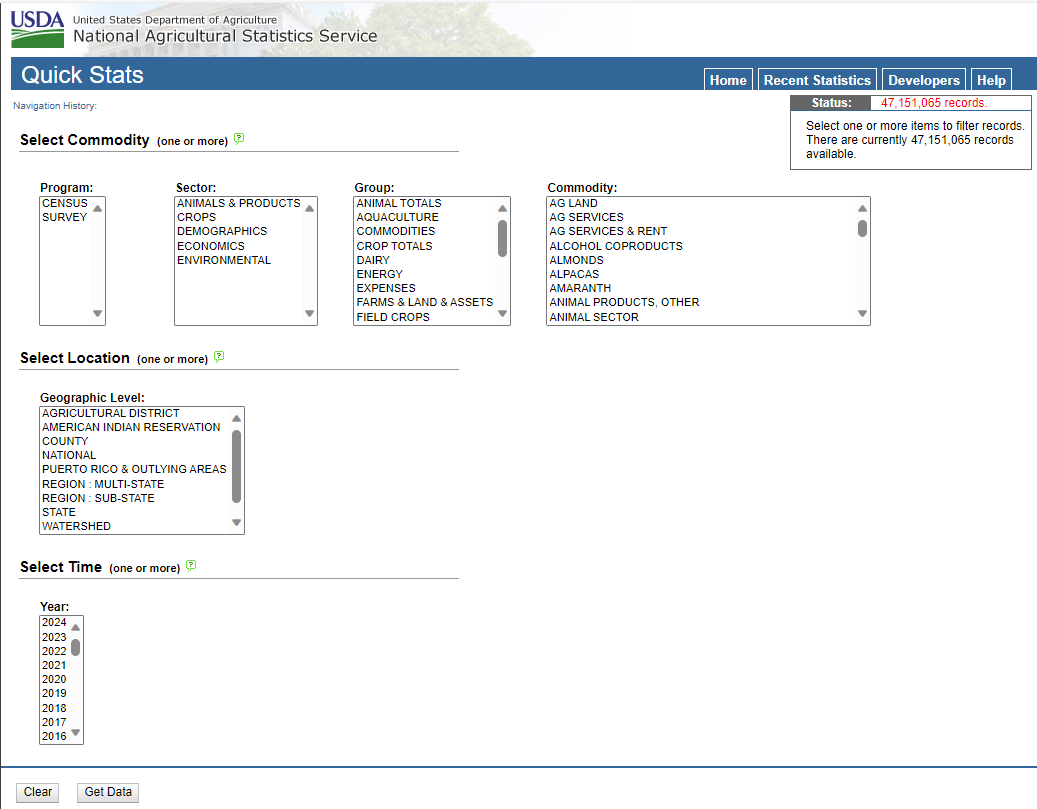
USDA National Agricultural Statistics Service Quick Stats
The United States Department of Agriculture's National Agricultural Statistics Service Quick Stats website is very nice. To date, You can download over 47 million rows of agricultural data to a csv file. So, let's buzz over there.
Query Criteria
Let's download a bit of data. We don't need a million rows for this demonstration. Let's download where
- Commodity = Honey
- Geographic Level = County
- State = Kentucky
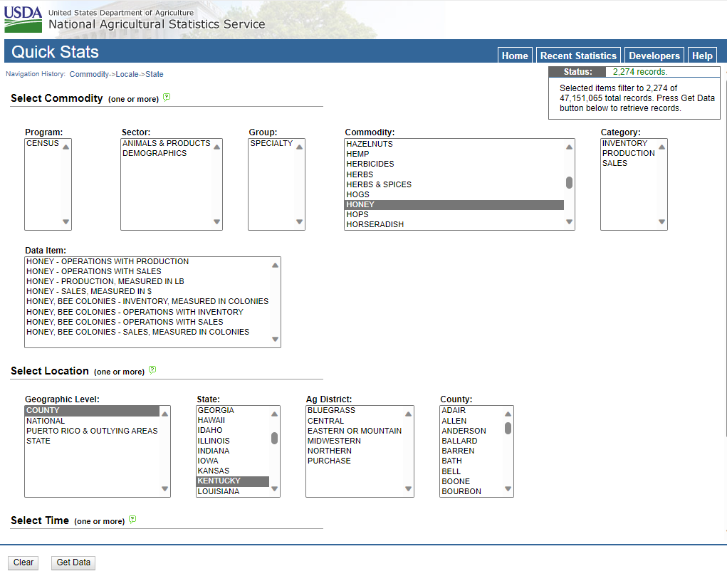
You can see that we will get 2,274 rows of data as of today. That's enough for today. Press the "Get Data" button.
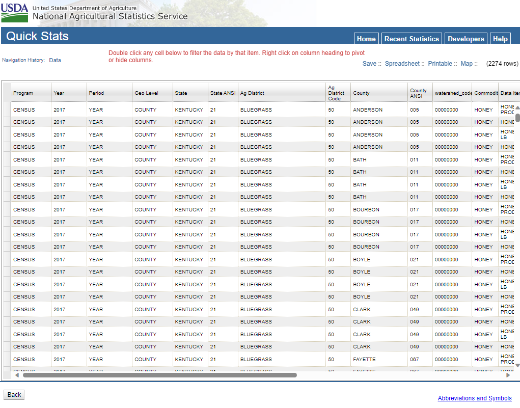
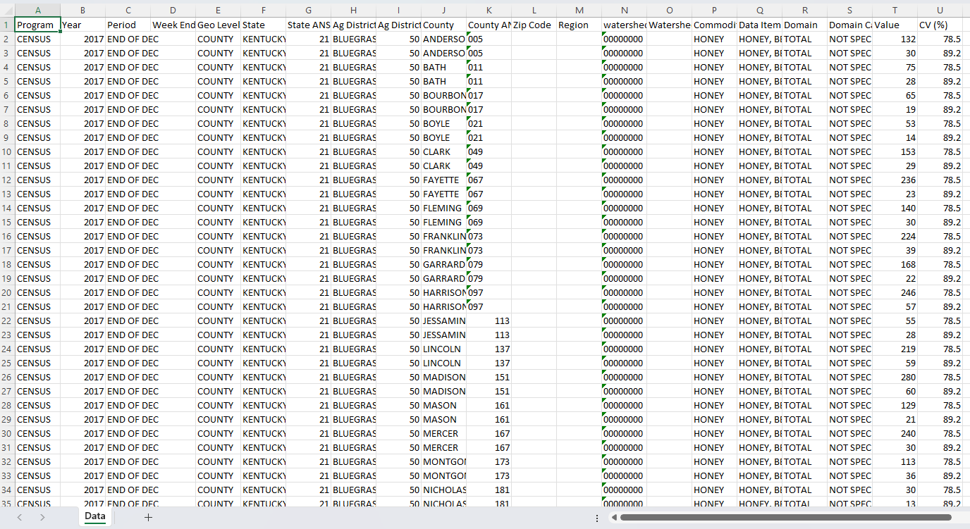
Press the "Spreadsheet" link at the top right, and the data will be downloaded to your local hard drive in a csv file. Open that file in Excel. Let's rename that sheet to "Data". Save the file as "Dynamic Arrays Example.xlsx". Our data should look like this:
Your first dynamic array
Before you can analyze your data, you must know what you have. We know that we have USDA data for Kentucky relating to Honey by County.
Let's create two sheets, "Dashboard" and "Reference". On Dashboard!B3 enter the formula:
=Data!A1:H15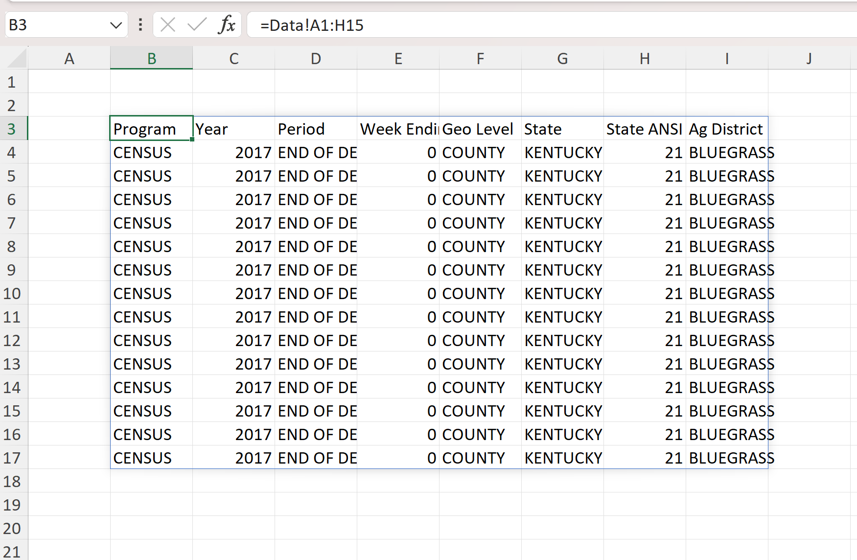
The formula is in B3, but the data goes from B3 to I17. All it does is pull the data from Data!A1:H15. Pretty simple. And very nice. You don't have to enter Data!A1 and copy/paste it to your desired cells.
You can't have any values where the returns. If you do, you will get a #SPILL! error. Whenever you get a #SPILL! error, you need to clear out some cells for your array to fit.
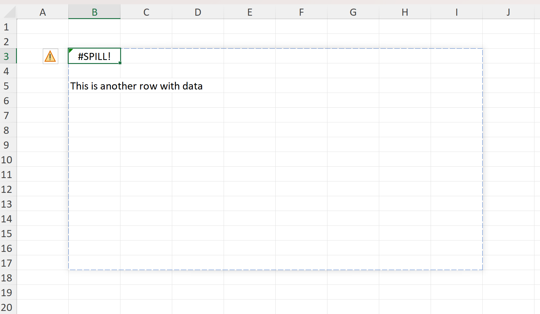
This is the simplest dynamic array. Let's kick it up a notch.
Unique and Sort
Without dynamic arrays, getting the unique values of a range was always a bit of a pain and, in my opinion, took too many steps. Now we can do it with the unique() function.
Let's determine how many unique values are in Data!Q2:Q2275 (remember we downloaded 2274 records with 1 header row). On the Dashboard sheet, enter "Data Item" in B3. Then in B4 enter:
=UNIQUE(Data!Q2:Q2275)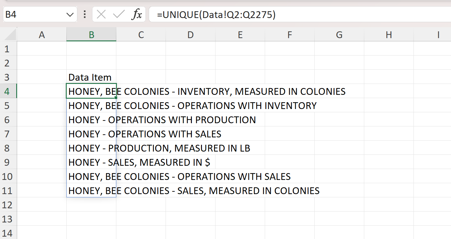
You will get back 8 records. They are the unique values of Data!Q2:Q2275. If you move to B5, you will see that the formula is "ghosted". If you enter something in B5, the formula in B4 will #SPILL!
There are 2 other parameters to the unique() function, one allows you to return unique columns or rows, the other one allows you to show distinct data. I've used this function since it came out. I've never used the other two parameters.
If we want to sort this data, we can close the unique() function with sort():
=SORT(UNIQUE(Data!Q2:Q2275))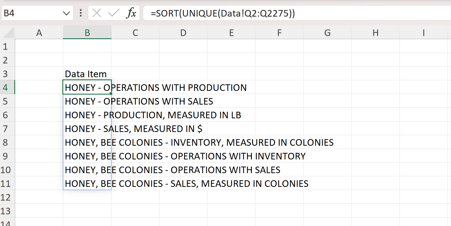
Pretty cool. This is perfect for a Reference sheet when allowing users to select a value from a dropdown list. I'll show you that in a future blog.
Now, let's prep for the next blog.
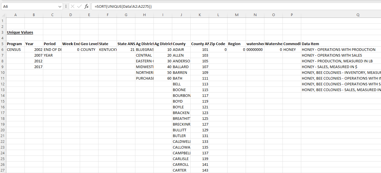
On the Reference sheet, cell A5 enter:
=Data!A1:S1Then bold A5:S5. Then in A6 enter:
=SORT(UNIQUE(Data!A2:A2275))and copy that to B6:S6. Now you have all of the unique values that we will use in future dynamic array blogs.
On the Dashboard sheet, cell A5, enter:
=Data!A1:U1and bold A5:U5. I've attached the file in case you need it.
In the next blog, we'll talk about the filter() function.


